Tutorial

Go through few examples.

First, import the following dependencies that we will be work with.

import numpy as np
from scipy.signal import ricker
from sweep_design import (ArrayAxis, Relation, Signal, UncalculatedSweep, 
                            ApriorUncalculatedSweep, Spectrum)
from sweep_design.utility_functions import tukey_a_t
import matplotlib.pyplot as plt 

Contents:

1. Introduction

2. ArrayAxis

3. Relation

4. Signal

5. Sweep

6. Spectrum

7. UncalculatedSweep

8. ApriorUncalculatedSweep

9. Configuration.

1. Introduction

The project was created for a simple design of sweep signal. Easy and fast way to create sweep signal. But to create a new one, we have developed a some new entities that help in creating of sweep signal.

Below representation structure of this objects in a project.

Following this diagram, we describe how to work with the library sweep-design.

2. ArrayAxis

Let’s create time axis. Start time is 0. end time is 10. sample of array 0.001

time = ArrayAxis(start=0., end=10., sample=0.001)

ArrayAxis has properties: size, actual_sample, start, end and sample

print(time.start)
print(time.end)
print(time.sample)
print(time.size)
print(time.actual_sample)

0.0
10.0
0.001
10001
0.0009999999999994458

Easy way to show information is print axis.

print(time)

start: 0.0
end: 10.0
sample: 0.001
size: 10001
calculated sample: 0.0009999999999994458

Calculated sample (time.actual_sample) - is sample taken from np.ndarray. Find common occurrence difference between neighbor of elements. The problem with floating numbers.

3. Relation

A relation instance is a representation of some mathematical functions, such as y = f(x).

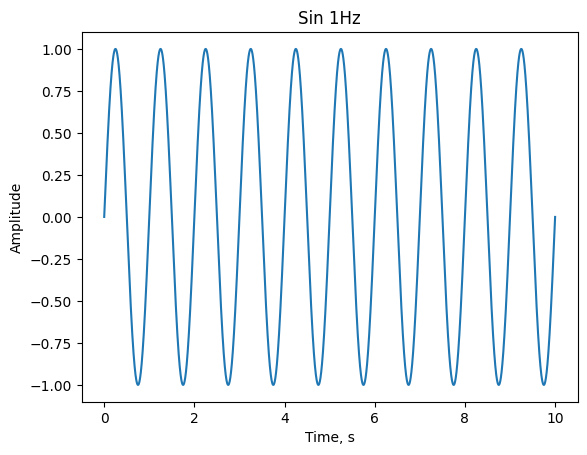
Look at building simple function of sin with frequency 1 Hz.

amplitude = np.sin(2*np.pi*time.array)
sin_1 = Relation(time, amplitude)

sin_1- instance of class Relation represent dependencies between time and amplitude such as mathematical function

\[ amplitude = sin(2\cdot\pi\cdot time) \]

Relation instance have same properties as ArrayAxis. Also have other properties: x, y.

We can use matplotlib to show result in next section.

r_time, r_amplitude = sin_1.get_data()
plt.plot(r_time, r_amplitude)
plt.xlabel('Time, s')
plt.ylabel('Amplitude')
plt.title('Sin 1Hz')

Text(0.5, 1.0, 'Sin 1Hz')

Also you can find maximum and minimum of relation

print(sin_1.max())
print(sin_1.min())

1.0
-1.0

Norm of function.

sin_1.get_norm()

5000.0

Interpolate of function expected by instance of Relation using new array axis

time_new = ArrayAxis(0.,10., 0.0005)
interpolate_sin_1 = sin_1.interpolate_extrapolate(time_new)

Shift relation, equal y=f(x+c) where c - is shift constant.

shifted_sin_1 = sin_1.shift(2)

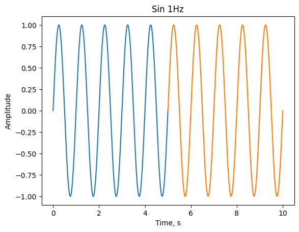
Also you can select interesting segment of data using to methods, select_data method or use square brackets.

r_time, r_amplitude = sin_1.get_data()
plt.plot(*sin_1.select_data(0., 5.).get_data())
plt.plot(*sin_1[5.:10.].get_data())
plt.xlabel('Time, s')
plt.ylabel('Amplitude')
plt.title('Sin 1Hz')

Text(0.5, 1.0, 'Sin 1Hz')

cumulative integration and differentiation of function

time_5 = ArrayAxis(-5., 5., 0.001)
y2 = Relation(time_5, time_5.array**2)
diff_y2 = y2.diff()
integration_y2 = y2.integrate()

plt.plot(*y2.get_data())
plt.plot(*diff_y2.get_data())
plt.plot(*integration_y2.get_data())
plt.xlabel('Time, s')
plt.ylabel('Amplitude')
plt.title('Functions')

Text(0.5, 1.0, 'Functions')

exponent of function. $\( y = f(x) \)\( \)\( r = e^y \)$ equal:

r = sin_1.exp()

With instance of class Relation we can use different mathematical operations (+, -, *, /, **, +=, -=, /=, *=). Operation can be with other instance of class Relation or numbers. Next examples with number. Subtraction constant from sin_1.

sub_sin_1 = sin_1-0.5
plt.plot(*sub_sin_1.get_data())
plt.xlabel('Time, s')
plt.ylabel('Amplitude')
plt.title('Sin 1Hz')

Text(0.5, 1.0, 'Sin 1Hz')

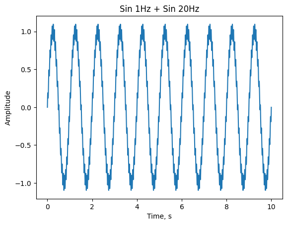
To demonstrate operation with other Relation instance, let’s create other sin function with 20Hz. And summing two instances sin_1 and sin_20.

sin_20 = Relation(time, 0.1*np.sin(time.array*2*np.pi*20))
sum_sin1_sin20 = sin_1 + sin_20

r_time_1_20, r_amplitude_1_20 = sum_sin1_sin20.get_data()
plt.plot(r_time_1_20, r_amplitude_1_20)
plt.xlabel('Time, s')
plt.ylabel('Amplitude')
plt.title('Sin 1Hz + Sin 20Hz')

Text(0.5, 1.0, 'Sin 1Hz + Sin 20Hz')

It’s better if you use a Relation instance with an equal axis array, but sometimes you can’t use. Then, when calculating math operation, new array axis found small sample and big boundaries. And y component of each relation interpolate with new common axis and extrapolate by zeros. After that, execute mathematical operation and return the result.

time1 = ArrayAxis(0., 7.5, 0.005)
time2 = ArrayAxis(2.5, 10., 0.001)

new_sin_1 = Relation(time1, np.sin(time1.array*2*np.pi))
new_sin_20 = Relation(time2, 0.1*np.sin(time2.array*2*np.pi*20))

new_sum_sin1_sin20 = new_sin_1 + new_sin_20

plt.plot(*new_sum_sin1_sin20.get_data())
plt.xlabel('Time, s')
plt.ylabel('Amplitude')
plt.title('New Sin 1Hz + Sin 20Hz')

Text(0.5, 1.0, 'New Sin 1Hz + Sin 20Hz')

To find two common axis for relations use class method equalize. This method use for math operations, convolution and correlations.

common_new_sin_1, common_new_sin_20 = Relation.equalize(new_sin_1, new_sin_20)

Available class methods to correlate and convolve. Look on convolution triangle and rectangle.

x = ArrayAxis(-1., 1., 0.001)

triangle = Relation(x, -1*(np.abs(x.array)-1))
rectangle = Relation(x, np.ones(x.size))

convolution = Relation.convolve(triangle, rectangle)

figure, axis = plt.subplots(2, 1, constrained_layout=True)

axis[0].plot(*triangle.get_data(), label='triangle')
axis[0].plot(*rectangle.get_data(), label='rectangle')
axis[0].set_title("figures")
axis[0].set_xlabel("X")
axis[0].set_ylabel("Y")
axis[0].legend()


axis[1].plot(*convolution.get_data())
axis[1].set_xlabel('X')
axis[1].set_ylabel('Convolution')
axis[1].set_title('Result Convolution')

Text(0.5, 1.0, 'Result Convolution')

4. Signal

The class Signal inherited from the class Relation. It has the same operation as Relation class. Additional has operation to convert signal to spectrum.

List additional methods:

signal_sin_1 = Signal(sin_1)
signal_sin_1.get_spectrum()
signal_sin_1.get_amplitude_spectrum()
signal_sin_1.get_phase_spectrum()
signal_sin_1.get_reverse_signal()
signal_sin_1.add_phase(signal_sin_1)
signal_sin_1.sub_phase(signal_sin_1)

<sweep_design.signal.Signal at 0x7f53fd9ec910>

and has properties: time and amplitude

print(signal_sin_1.time)
print(signal_sin_1.amplitude)

start: 0.0
end: 10.0
sample: 0.001
size: 10001
calculated sample: 0.0009999999999994458
[ 0.00000000e+00  6.28314397e-03  1.25660399e-02 ... -1.25660399e-02
 -6.28314397e-03 -2.44929360e-15]

Let’s check that the sum of sin 1 Hz and 20 Hz has an amplitude spectrum of 1 Hz and 20 Hz.

signal_sum_sin1_sin20 = Signal(sum_sin1_sin20)
plt.plot(*signal_sum_sin1_sin20.get_amplitude_spectrum()[0:50].get_data())
plt.xlabel('Frequency, Hz')
plt.ylabel('Amplitude')
plt.title('Amplitude spectrum Sin 1Hz + Sin 20Hz')

Text(0.5, 1.0, 'Amplitude spectrum Sin 1Hz + Sin 20Hz')

Where an operation with signal is expected, the spectrum instance will be converted to signal instance and operation will be with them.

5. Spectrum

The Spectrum class inherited from Relation class. It has the same operation as Relation class. Additional has operation to convert spectrum to signal.

List additional methods:

spectrum_sum_sin1_sin20 = signal_sum_sin1_sin20.get_spectrum()
spectrum_sum_sin1_sin20.get_amp_spectrum()
spectrum_sum_sin1_sin20.get_phase_spectrum()
spectrum_sum_sin1_sin20.get_reverse_filter()
spectrum_sum_sin1_sin20.add_phase(spectrum_sum_sin1_sin20)
spectrum_sum_sin1_sin20.sub_phase(spectrum_sum_sin1_sin20)

<sweep_design.spectrum.Spectrum at 0x7f53fac50290>

Class method get_spectrum_from_amp_phase

amplitude_spectrum = spectrum_sum_sin1_sin20.get_amp_spectrum()
phase_spectrum = spectrum_sum_sin1_sin20.get_phase_spectrum()

spectrum = Spectrum.get_spectrum_from_amp_phase(amplitude_spectrum, phase_spectrum)

Where an operation with spectrum is expected, the signal instance will be converted to spectrum instance and operation will be with them.

6. Sweep

The Sweep class represent of sweep function. Sweep inherited from the Signal class. And the Sweep class has the same methods as Signal class.

Also Sweep instance has next properties:

• frequency_time - frequency modulation

• amplitude_time - amplitude modulation

• spectrogram - spectrogram of sweep signal. Expected by class Spectrogram

• a_prior_signal - the signal from which the sweep signal created, or None.

If create sweep instance directly from some signal, then frequency_time and amplitude_time functions will be calculated using hilbert transformation from scipy.

How properties look in the following sections.

7. UncalculatedSweep

UncalculatedSweep is class to create Sweep instance.

The construction of a sweep signal is carried out according to the formula:

\[ S(t) = A(t)sin(\theta(t)+\theta_0) \]

where \(t\) is the time that varies within \([0, T]\) \(A(t)\) is the sweep amplitude change function, \(\theta(t)\) is the angular sweep, \(\theta_0\) is the initial phase

\[ \theta(t) = 2\pi\int\limits_{0}^{t}F(\tau)d\tau \]

where \(F(t)\) - frequency versus time

UncalculatedSweep take three parameters:

• time,

• amplitude_time function or amplitude modulation,

• frequency_time function or frequency modulation,

Analytic functions (frequency_time and amplitude_time) can be as array of numbers or as callable object(lambda function, common python functions and ect.) Example: frequency_time = lambda t: t*10+1, amplitude_time = lambda t: np.ones(t.size)

time is ArrayAxis, or np.ndarray (array of numbers), or None

To get instance of Sweep, we should call instance of UncalculatedSweep with a new or same time axis or with None. If we call with None, function tries to use time when we created instance UncalculatedSweep. If time was is not found then an exception will raised.

time_sweep = ArrayAxis(0.,10.,0.001)
unsw = UncalculatedSweep(time_sweep, lambda time: 10*time+1, lambda time: np.ones(time.size))
linear_sweep = unsw()

plt.plot(*linear_sweep.get_data())
plt.xlabel('Time, s')
plt.ylabel('Amplitude')
plt.title('Linear sweep')

Text(0.5, 1.0, 'Linear sweep')

Show function time frequency:

plt.plot(*linear_sweep.frequency_time.get_data())
plt.xlabel('Time, s')
plt.ylabel('Frequency, Hz')
plt.title('Frequency function')

Text(0.5, 1.0, 'Frequency function')

Show function amplitude time:

plt.plot(*linear_sweep.amplitude_time.get_data())
plt.xlabel('Time, s')
plt.ylabel('Amplitude')
plt.title('Amplitude function')

Text(0.5, 1.0, 'Amplitude function')

Image of Spectrogram:

time_spectrogram = linear_sweep.spectrogram.time
frequency_spectrogram = linear_sweep.spectrogram.frequency
extent = [
    time_spectrogram.start, 
    time_spectrogram.end, 
    frequency_spectrogram.start, 
    frequency_spectrogram.end
]
plt.xlabel("Time, s")
plt.ylabel("Frequency, Hz")
plt.title("Spectrogram linear sweep")
plt.imshow(linear_sweep.spectrogram.spectrogram, extent=extent, aspect='auto')

<matplotlib.image.AxesImage at 0x7f53fa7b26d0>

Next example.

As a change in frequency over time, we take the function:

\[F(t) = sin(2\pi t/2)/2\cdot9+1 \]

where \(t\) - time

It is described below as a function f_t.

As a change in the amplitude envelope with time, we take the Tukey window function, in N samples

\[\begin{split} w[n] = \begin{cases} \frac{1}{2}[1-cos(\frac{2\pi n}{\alpha N})], & 0 \le m < \frac{\alpha N}{2} \\ 1, & \frac{\alpha N}{2} \le t < \frac{N}{2} \\ w[N-n], & 0 \le n \le \frac{N}{2} \end{cases} \end{split}\]

where \(n\) - sample, \(N\) - total samples, \(\alpha\) - coefficient from 0 to 1

By using the tukey function from the scipy library. Specifying the number of samples as the length of the array along the time axis and taking \(\alpha\) = 0.3.

It is described below as a function of a_t.

def f_t(time: np.ndarray) -> np.ndarray:
    return (np.sin(time * 2 * np.pi / 2) + 1) / 2 * 9 + 1


usw = UncalculatedSweep(time=time_sweep, frequency_time=f_t, amplitude_time=tukey_a_t(time_sweep.array, 1))
sw = usw()


plt.plot(*sw.get_data())
plt.xlabel('Time, s')
plt.ylabel('Amplitude')
plt.title('Linear sweep')

Text(0.5, 1.0, 'Linear sweep')

plt.plot(*sw.frequency_time.get_data())
plt.xlabel('Time, s')
plt.ylabel('Frequency, Hz')
plt.title('Frequency function')

Text(0.5, 1.0, 'Frequency function')

plt.plot(*sw.amplitude_time.get_data())
plt.xlabel('Time, s')
plt.ylabel('Amplitude')
plt.title('Amplitude function')

Text(0.5, 1.0, 'Amplitude function')

time_spectrogram = sw.spectrogram.time
frequency_spectrogram = sw.spectrogram.frequency
extent = [
    time_spectrogram.start,
    time_spectrogram.end,
    frequency_spectrogram.start,
    frequency_spectrogram.end
]
plt.xlabel("Time, s")
plt.ylabel("Frequency, Hz")
plt.title("Spectrogram sin sweep")
plt.imshow(sw.spectrogram.spectrogram, extent=extent, aspect='auto')

<matplotlib.image.AxesImage at 0x7f53fa6cc910>

8. ApriorUncalculatedSweep

Construction of a sweep signal from a priori data.

There is another possibility of building a sweep signal using a priori data.

To do this, you need to use the ApriorUncalculatedSweep class. This class inherits from UncalculatedSweep.

The difference lies in the arguments it takes to construct an instance of the class:

1. The first argument time is responsible for a time.

2. The second argument is responsible for a priori data, it can be an instance of a class: Relation, Signal, Spectrum or Sweep.

3. The third argument is responsible for the method (function), with the help of which functions or sequences of frequency versus time and amplitude versus time will be extracted.

The extracted functions (amlitude_time, frequency_time) will then be passed to the superclass UncalculatedSweep.

Further calling an instance of the ApriorUncalculatedSweep class is similar to calling an instance of the UncalculatedSweep class, which returns an instance of the Sweep class.

Consider an example of obtaining a sweep signal from a Reeker impulse. We will also use the function to receive a signal from the scipy library.

time_ricker = ArrayAxis(0., 1., 0.0002)
amplitude_ricker = ricker(time_ricker.size, a=2)
ricker_signal = Signal(time_ricker, amplitude_ricker)
plt.plot(*ricker_signal[0.475:0.525].get_data())
plt.xlabel('Time, s')
plt.ylabel('Amplitude')
plt.title('Ricker signal')

Text(0.5, 1.0, 'Ricker signal')

time_sweep_2 = ArrayAxis(0.,10., 0.0002)
usw2 = ApriorUncalculatedSweep(time=time_sweep_2, a_prior_data=ricker_signal)
sw2 = usw2()

The ftat_method parameter is optional. The default function is simple_freq2time from Config class sweep_design.config

def simple_freq2time(spectrum: 'Spectrum') -> Tuple[np.ndarray, np.ndarray, np.ndarray]:
    f, A = spectrum.get_amp_spectrum().get_data()
    n_spec = A ** 2
    nT = np.append([0.], ((n_spec[1:]+n_spec[:-1])/(f[1:]-f[:-1])).cumsum())
    coef = integrate.trapz(n_spec, f)
    a_t = sqrt(coef*2)*np.ones(len(nT))
    return nT, f, a_t

plt.plot(*sw2.get_data())
plt.xlabel('Time, s')
plt.ylabel('Amplitude')
plt.title('Sweep-signal')

Text(0.5, 1.0, 'Sweep-signal')

aprior_signal = sw2.a_prior_signal
plt.plot(*aprior_signal[.475:.525].get_data())
plt.xlabel('Time, s')
plt.ylabel('Amplitude')
plt.title('A prior signal')

Text(0.5, 1.0, 'A prior signal')

The result is a non-linear sweep signal whose amplitude spectrum is similar to the amplitude spectrum of the transmitted spectrum of the Reeker signal.

You can verify this by using the execution of sequences of functions:

1. On instances of the Sweep and Signal classes, which are sw2 and aprior_signal, you can call the get_amplitude_spectrum() method, which returns an instance of the class Relation describing the amplitude spectrum of the signals.

2. And finally, as in the previous examples, retrieve the data using the get_data() method and pass the result to the plt.plot() method

norm_sweep = sw2.get_norm()
freq_f_t2, amp_f_t2 = sw2.get_amplitude_spectrum().get_data()
plt.plot(freq_f_t2, amp_f_t2, label="Sweep from Ricker")
freq_f_t3, amp_f_t3 = ricker_signal.get_amplitude_spectrum().get_data()
plt.plot(freq_f_t3, amp_f_t3, label="Ricker")
plt.xlabel('Frequency, Hz')
plt.ylabel('Amplitude')
plt.title('Amplitude Spectrum')
plt.legend()

<matplotlib.legend.Legend at 0x7f53fa6fccd0>

9. Config

If you don’t like default methods that calculated new parameters, you can override the methods in the Config and the ConfigSweep classes, which are located in the sweep_design.config module. See API References. for more information.

Next section you can find examples of prepared sweep.

10. Utility functions and prepared sweeps

Module sweep-design.utility_functions contains functions:

• tukey_a_t - for amplitude modulation.

• get_IMFs_ceedman and get_IMFs_emd - empirical mode decomposition.

• f_t_linear_array and f_t_linear_function - linear frequency modulation.

• proportional_freq2time and dwell - extractor frequency modulation and amplitude modulation from Spectrum.

• correct_sweep - correction sweep for displacement.

• get_correction_for_source - correction sweep for displacement using limitation of source.

Module sweep-design.prepared_sweep contains functions to create sweep:

• get_dwell_sweep - extract dwell sweep signal from a prior Spectrum.

• get_linear_sweep - get_linear_sweep from a prior Spectrum

• get_shuffle - get shuffle sweep.

• get_code_sweep_segments - get sweep by composing sweep signal in sequence of set code.

• get_convolution_sweep_and_code - get sweep by correlate sweep and code.

• get_m_sequence_code, get_relation_m_sequence - m-sequence code.

• get_code_zinger, get_code_zinger_relation - extract zinger code.